Your Token is a Wonderland

What would it look like to train a transformer on the most personal dataset possible — your own private conversations — and then actually look inside it?

The idea arrived at dinner with my wife, Francisco, and Jamie at our favorite spot in Los Angeles. We'd been talking about how much of a language model's behavior comes not from pre-training or post-training, but from context alone — about tokens as the fundamental unit of identity inside these systems.

I called it Your Token is a Wonderland.

The joke is obvious — the John Mayer song — but the meaning underneath it isn't really a joke. Your tokens are, in a precise technical sense, a wonderland: a high-dimensional space full of structure that was put there by your habits, your vocabulary, your psychology, without you ever intending to build anything. And if you train a model on that space and then look inside the model, you are not reading a summary of yourself. You are reading the circuits that gradient descent invented to predict you.

I went home, started reading, and didn't really stop. I spent the next two weekends deep in mechanistic interpretability — the Anthropic transformer circuits work, the induction heads paper, the superposition research — and then a week actually running the experiments.

What follows is a practitioner's field notes, with all the wrong turns included: extracting iMessage data from macOS, training a small transformer from scratch, and running a full interpretability pipeline to find the circuits the model learned.

This is not a research paper. I'm someone with a product background, a lot of curiosity, and two free weekends. The findings are real and some of them are genuinely surprising for a model this small. The methodology is reproducible by anyone with a Mac, an AWS account, and enough stubbornness to push through.

Why Personal Data

Most mechanistic interpretability work happens on GPT-2, or on toy models trained on synthetic sequences, or on large proprietary models where you have limited access to internals. These are the right choices for rigorous research. But for someone trying to learn interpretability, they have a problem: you're studying a model predicting tokens you don't intimately know.

Your own text messages are different. You have ground truth from lived experience. When the model generates "sounds good" after "what time works for you?", you know whether that's in-character. When a head seems to track who is speaking, you can verify it because you were there for every conversation. The familiarity is an analytic advantage.

There's also something philosophically interesting about the question. A transformer trained on your iMessage corpus has, in some weak sense, learned a statistical model of your communication patterns — your vocabulary, your rhythms, your topic preferences, your emotional register. What is that, exactly? What circuits did it need to build to predict you? That question drove two weekends of reading and one week of running experiments.

The Setup

The Pipeline

The project has six stages:

Extract the iMessage database and decode the binary message format
Filter out automated messages and noise
Train the BPE tokenizer and transformer
Run sanity checks before committing to expensive analysis
Generate interactive visualizations to identify components worth investigating
Run hypothesis testing and circuit analysis on components that survived triage

The code isn't open yet — if there's interest, I'm happy to clean things up and get it ready for sharing.

Hardware: Local vs. Cloud

The most consequential practical decision was the local/cloud split. Use local machines for fast iteration (tokenizer training, sanity checks, visualization, interpretation) and cloud for the GPU-intensive step (model training).

Tokenizer training runs locally (MacBook Air M1). The BPE tokenizer trains in under a minute regardless of corpus size. Always do this step locally so you can verify the output before committing to a multi-hour training run.

Model training should run in the cloud. I initially tried training locally and watched the progress bar crawl. At 332,000 training examples, 10 epochs on MPS took roughly 3 days. The same run on an AWS g6.xlarge instance (NVIDIA L4 GPU) completed under 90 minutes. The full training run — including the extended run to 20 epochs — cost under $5.

Tokenizer

The thing I burned the most hours debugging is that special tokens must be registered during tokenizer training, not added afterward. The special tokens are <|me|>, <|them|>, <|sep|>, <|endoftext|>, and <|pad|>.

When registered at training time, the BPE algorithm treats them as atomic units that merges can never cross. When added afterward, they get split by the existing merge rules into sub-tokens — <|me|> becomes [<|, me, |>] and the model cannot learn a clean speaker-tracking circuit because the speaker signal is spread across three ambiguous positions.

Two additional gotchas:

The add_special_tokens() call when loading saved tokenizer files is not mentioned in the HuggingFace tokenizers documentation but is essential — without it, special tokens are split by BPE even if they were registered at training time.
Uploading stale tokenizer files from a previous failed attempt will silently overwrite the good ones. Keep the AWS instance as the source of truth for tokenizer files.

I made it a point to run verification before every training run:

<|endoftext|>    id=[0]   ✓
<|me|>           id=[1]   ✓
<|them|>         id=[2]   ✓
<|sep|>          id=[3]   ✓
<|pad|>          id=[4]   ✓

Model Architecture

Parameter	Value	Reasoning
Layers	4	Small enough to name every component
Heads	4	16 total — fully traceable
d_model	256	Interpretable residual stream dimension
d_mlp	1024	Standard 4× expansion
Context length	128	Covers most iMessage exchanges
Parameters	5.3M	Small enough for full interpretability

The model is implemented using TransformerLens, which is the standard library for mechanistic interpretability work. It exposes every internal activation through a hook system, which is what makes the patching analysis possible later.

One note: torch.compile with TransformerLens requires mode=None (the default), not mode="reduce-overhead". The reduce-overhead mode enables CUDAGraphs, which is incompatible with TransformerLens's hook infrastructure. This produces a cryptic accessing tensor output of CUDAGraphs error that is not obviously related to the compile mode.

The Data

Extraction: The Binary Blob Problem

macOS stores iMessages in a SQLite database at ~/Library/Messages/chat.db. The database has a text column that you'd expect to contain the message text. In my database, it did — for about 0.3% of messages. The other 99.7% store content in a column called attributedBody, which is a binary blob in NeXTSTEP typedstream format, a serialization format that predates macOS and is sparsely documented. Most tutorials and blog posts about chat.db work with the text column directly and silently operate on a tiny fraction of the actual corpus.

Decoding it required implementing a typedstream parser using the macOS Foundation framework via PyObjC. Terminal also needs Full Disk Access to read chat.db — a macOS security requirement that has silently broken more than one attempt at this. Once both were handled, extraction was clean.

Loaded 722772 messages from messages.jsonl

=== Extraction Results ===
Total messages:           722772
  From you:               281873  (39%)
  From others:            440899  (61%)
  In group chats:         146206
  SMS:                    8855

Unique contacts:          1016
Total words:              5560798
Avg words/msg:            7.7

Files written:
  messages.jsonl
  corpus.txt
  corpus_threaded.txt  (181044 windows)
  corpus_me_only.txt

The corpus was formatted as threaded conversation windows — 8 messages at a time with a stride of 4, tagged with speaker tokens:

<|them|> are you free tomorrow? <|sep|>
<|me|> yeah totally works <|sep|>
<|them|> great see you at noon <|endoftext|>

Filtering

Five categories of noise were removed:

Automated messages (OTPs, shipping notifications, banking alerts)
Short-code senders
URL-only messages
Pure emoji
Profanity

I removed profanity as a precaution for training stability and corpus cleanliness. In retrospect it made no meaningful difference to model quality — the removed messages were less than 1% of the corpus. The generation problems I encountered later were architectural, not vocabulary.

The model and all intermediate data remained on my local machine and the AWS training instance. Nothing was shared or published, and the model itself was deleted after analysis.

Training

Training ran for 20 epochs:

Epoch	Loss	What's happening
0	~6.2	Model knows nothing
3	~4.1	Learned basic token statistics
9	~3.02	First checkpoint — functional but shallow
14	~2.90	Diminishing returns beginning
19	~2.83	Converged — final checkpoint

Final loss of 2.83 corresponds to a perplexity of about 17 — the model is typically uncertain among 17 candidates for the next token. Far from random (which would be loss ~8.3 over the 4,096-token vocabulary) but far from deterministic. The plateau from epoch 14 onward is the 5.3M parameter budget hitting its ceiling. Further training wouldn't help without a larger architecture.

The Interpretability Pipeline

Before explaining the findings, a brief framing of what mechanistic interpretability is trying to do. A transformer is a mathematical function with millions of learned parameters. We know what it does — predict the next token — but not how. The goal of mech interp is to reverse-engineer the internal computations: find the specific components (attention heads, MLP neurons) responsible for specific behaviors, understand what those components are computing, and verify causal claims with controlled experiments.

The tools for this are: activation patching, attention pattern analysis, OV circuit decomposition, and causal scrubbing. I'll explain each as they come up.

Triage: Finding the Needle

The first stage is triage — running a broad set of analyses to identify which components are worth investigating deeply. The pipeline generates eight interactive HTML visualizations.

Four of them are for initial screening:

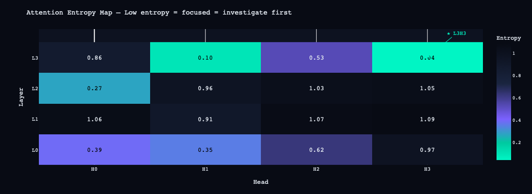
1. Entropy map — Shannon entropy of each head's attention distribution. Low entropy means focused attention (a specific job); high entropy means diffuse mixing. Six of sixteen heads showed focused patterns: L0H0, L0H1, L2H0, L3H1, L3H2, L3H3. The concentration in L0 and L3 suggested those layers were doing specialized work.

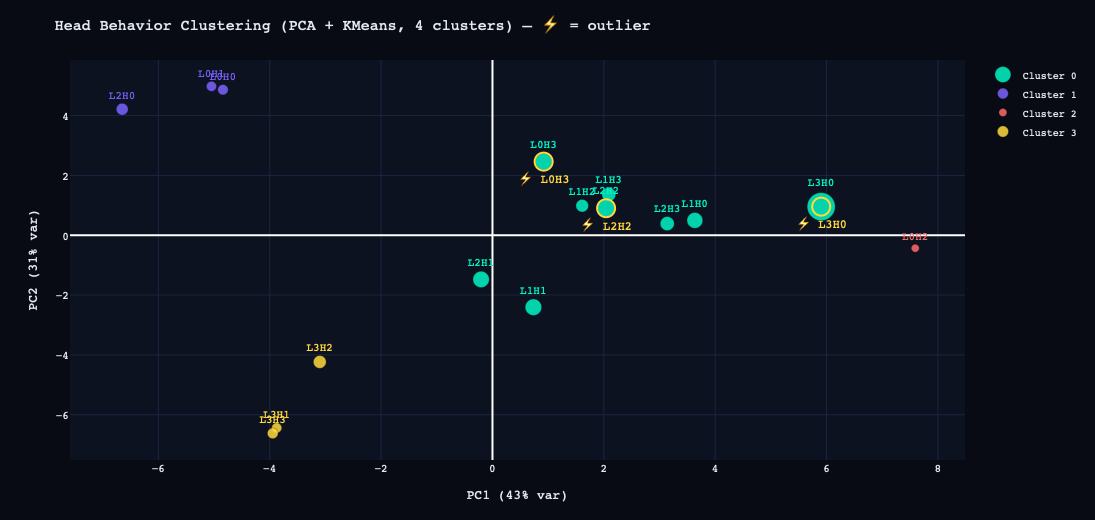
2. Head clustering — Each head represented as a feature vector, projected to 2D via PCA and clustered with KMeans. Top outliers: L3H0, L2H2, L0H3, L1H1. These became secondary targets.

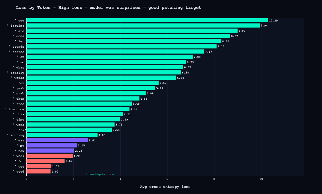
3. Loss by token — Per-token cross-entropy loss across sample prompts. The most surprising tokens were all sentence-initial content words: see (10.29), leaving (9.94), are (8.99). This makes sense: given <|me|>, the model has established speaker identity but the specific word that follows is highly variable. The model is most uncertain at exactly the positions where speaker-specific style would manifest.

4. Residual stream PCA — Token trajectories through layers projected to 2D. A large jump between layers means that layer is doing substantive work on that token.

Activation Patching Grid (The Needle-Finder)

This is the most important visualization in the pipeline.

How it works: Two prompts are defined — a "clean" prompt (the behavior you want to understand) and a "corrupted" prompt (a minimally different prompt that produces different behavior). The model runs on both. Then, for each (layer, token position) pair, the activation from the clean run is patched into the corrupted run. If the model recovers the clean behavior, that (layer, position) is causally responsible for the difference.

My prompts:

Clean: <|me|> yeah totally works for me
Corrupted: <|me|> nah nothing works for me
Target token: the final word

The grid was run in three modes — resid_pre (full residual stream), attn_out (attention only), mlp_out (MLP only). The results were sharp:

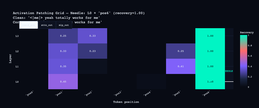
resid_pre: the entire pos6 column lights up at recovery 1.00 across all layers. By the time computation reaches the final position, the behavior is fully determined.

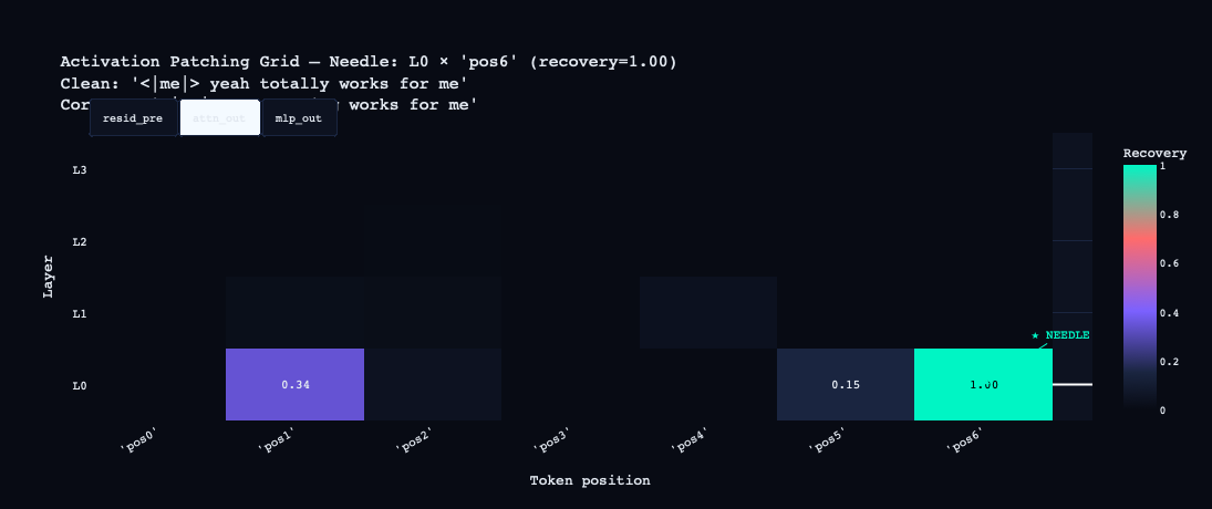
attn_out: L0 at pos6 = 1.00. Layer 0 attention, reading from the final token position, is causally sufficient on its own. Everything else is near zero.

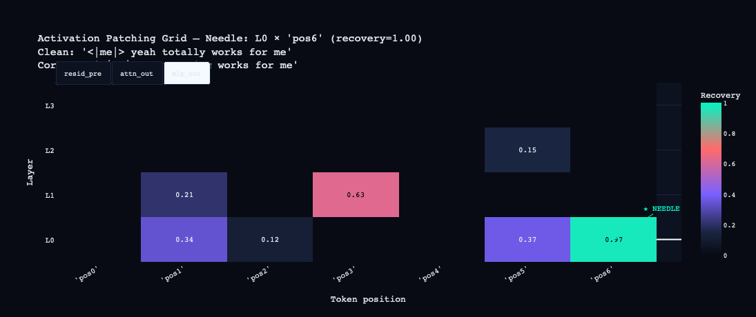
mlp_out: L1 at pos3 = 0.63. Position 3 is the word "works" in the clean prompt. The layer 1 MLP is doing significant computation at that content word — likely encoding something about verb-completion context.

The circuit story this suggests: L0 attention at the final position handles the primary computation, with L1 MLP contributing semantic context at the verb.

Logit Lens, OV Circuit, Circuit Graph

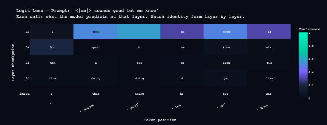
The logit lens projects the residual stream at each layer through the unembedding matrix to show what the model would predict at that point. Watching predictions form layer by layer is one of the most visually interpretable outputs of the pipeline — you can see the model's "confidence" about the final token build as computation proceeds.

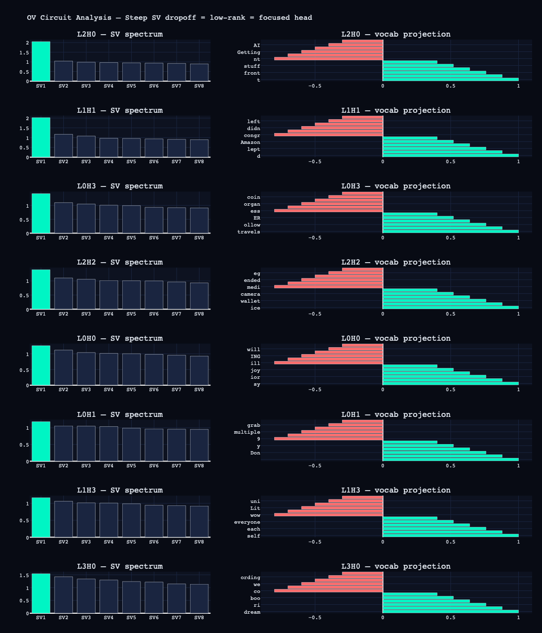
The OV circuit for each head is computed as W_V @ W_O. SVD of this matrix reveals how many distinct "jobs" a head performs — a steep singular value dropoff (SV1 >> SV2) means the head is essentially doing one thing. The vocabulary projection of the top singular vector names what that thing is.

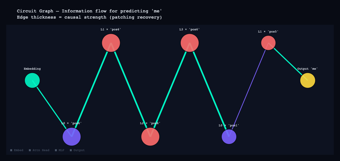
The circuit graph pulls all the patching results into a single directed graph. Nodes are components — attention heads and MLP layers — and edges represent causal influence, weighted by recovery score. What emerges is a readable map of how information flows through the model for a given prediction: which components contribute, which ones feed into which, and where the critical path lies.

The Findings

Finding 1: The Cooperative L0H0+L0H1 Circuit

The first hypothesis tested with causal scrubbing was the L0 circuit identified by the patching grid.

Causal scrubbing works as follows: patch only the hypothesized circuit components (clean activations into the corrupted run), leave everything else corrupted, and measure how much behavior is recovered. Recovery > 0.8 is considered sufficient evidence that the hypothesized circuit is causally responsible.

Results with circuit [(0, 0), (0, 1)]:

Full circuit patching:
  Recovery: 0.875   ✓ SUFFICIENT (>0.8)

Per-head contribution:
  L0H0:  -2.711
  L0H1:  -1.904

Leave-one-out:
  Without L0H0: recovery = -3.509   ← NECESSARY
  Without L0H1: recovery = -3.145   ← NECESSARY

The recovery number says the circuit is sufficient. But look at the per-head contributions — both are strongly negative. Patching L0H0 alone makes things worse by 2.7. Patching L0H1 alone makes things worse by 1.9. Yet patching both together recovers 87.5% of the behavior.

The most natural explanation is superposition — the feature is distributed across both heads in a way that requires both vectors to reconstruct it. Remove either one and you don't get half the feature — you get noise, because the remaining head is carrying a component of something that doesn't make sense without its partner. Though it's worth noting that the negative individual recoveries could also be an artifact of the patching methodology itself: inserting one clean activation into an otherwise corrupted run creates an inconsistent internal state that may perform worse than a fully corrupted one.

If it is superposition, the mechanism would be: the model has a 256-dimensional residual stream and needs to represent thousands of features. The solution is to pack multiple features into overlapping directions — mathematically possible because the features are rarely active simultaneously. Individual heads become entangled in each other's representations. This is what Anthropic's superposition research predicted, and it would be striking to see it in a 5M parameter model trained on text messages. But confirming it requires more targeted experiments than activation patching alone can provide.

Finding 2: L3H3 — The Speaker-Tracking Head

L3H3:
  Pattern:    first_token  (first=0.99, prev=0.19, entropy=0.04)
  OV:         promotes=[' cred', ' Th', 'ales']
  Ablation:   delta_loss = +0.1179  (high)

Entropy of 0.04 is extremely low — this head attends to position 0 with 99% probability on every forward pass, regardless of what the rest of the sequence contains. Position 0 is always the speaker token: <|me|> (id=1) or <|them|> (id=2).

L3H3 is a late-layer head (layer 3 of 4) with a single, extreme specialization: read the speaker token and ignore everything else. The structural comparison with L3H1 (entropy=0.10, first=0.98) shows a pattern: the model has evolved two late-layer heads that both lock onto speaker identity, with slightly different specificity. These are the heads that enforce the distinction between "Kunal's style" and "everyone else's style" in the final layer of computation before the unembedding.

Nobody programmed this specialization. It emerged because the model discovered that speaker identity is one of the highest-leverage features for predicting what comes next in a conversation. Given <|me|>, the distribution over next tokens is your personal vocabulary distribution. Given <|them|>, it's the aggregate vocabulary of 200+ different people you've texted. Dedicating a head to reading this distinction is one of the highest-ROI investments the model could make.

Finding 3: L0H2 — The Only Structural Head

L0H2:
  Pattern:    prev_token  (first=0.35, prev=0.76, entropy=0.62)
  OV:         promotes=[' Karebear', ' 30', ' valley']
  Ablation:   delta_loss = +0.6192  (high — third highest in model)

L0H2 attends to the previous token 76% of the time. It sits in layer 0, which means it runs before any other computation. And its ablation impact (+0.619) is one of the highest in the entire model — removing it degrades performance significantly.

This is a previous-token head, and it serves a specific structural purpose: ensuring that every position knows what came before it. Think of it as a relay mechanism. Token at position 5 needs information from position 4 to make a good prediction. L0H2 is the dedicated circuit for making that information available.

What makes this noteworthy is that previous-token heads appear in essentially every transformer that has been analyzed, from toy models to GPT-2 to large production models. The fact that one appears in a 5M parameter model trained on your personal text messages is a small piece of evidence for a larger claim: certain computational primitives are so universally useful for sequential prediction that any network trained on sequential data will independently invent them. The model didn't copy this structure from GPT-2 — it discovered it from scratch because it's the right solution to the information-routing problem.

Finding 4: 98-100% Polysemanticity

MLP Layer 0:  monosemantic=0 (0%)    polysemantic=63 (98%)   mixed=1 (2%)
MLP Layer 1:  monosemantic=0 (0%)    polysemantic=64 (100%)  mixed=0 (0%)
MLP Layer 2:  monosemantic=0 (0%)    polysemantic=63 (98%)   mixed=1 (2%)
MLP Layer 3:  monosemantic=0 (0%)    polysemantic=60 (94%)   mixed=4 (6%)

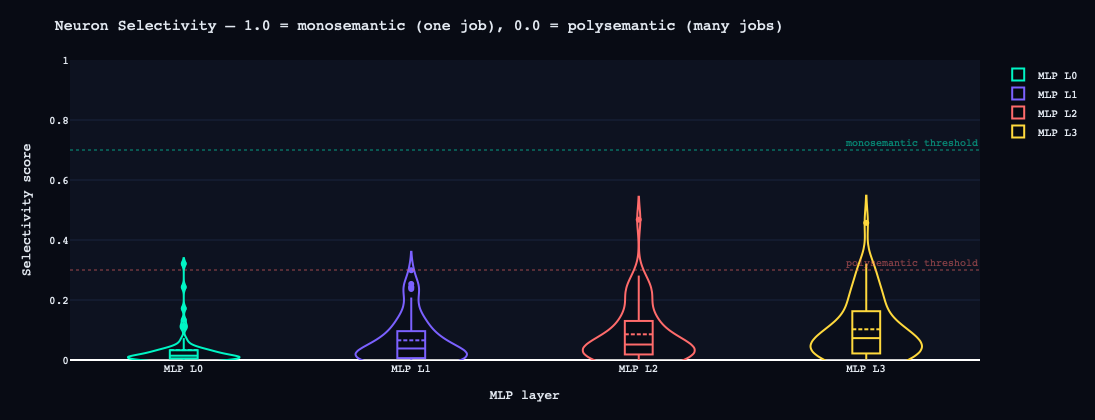
A monosemantic neuron fires strongly for one semantic category and weakly for others. A polysemantic neuron fires for multiple unrelated categories with similar intensity. Every MLP layer in this model is overwhelmingly polysemantic.

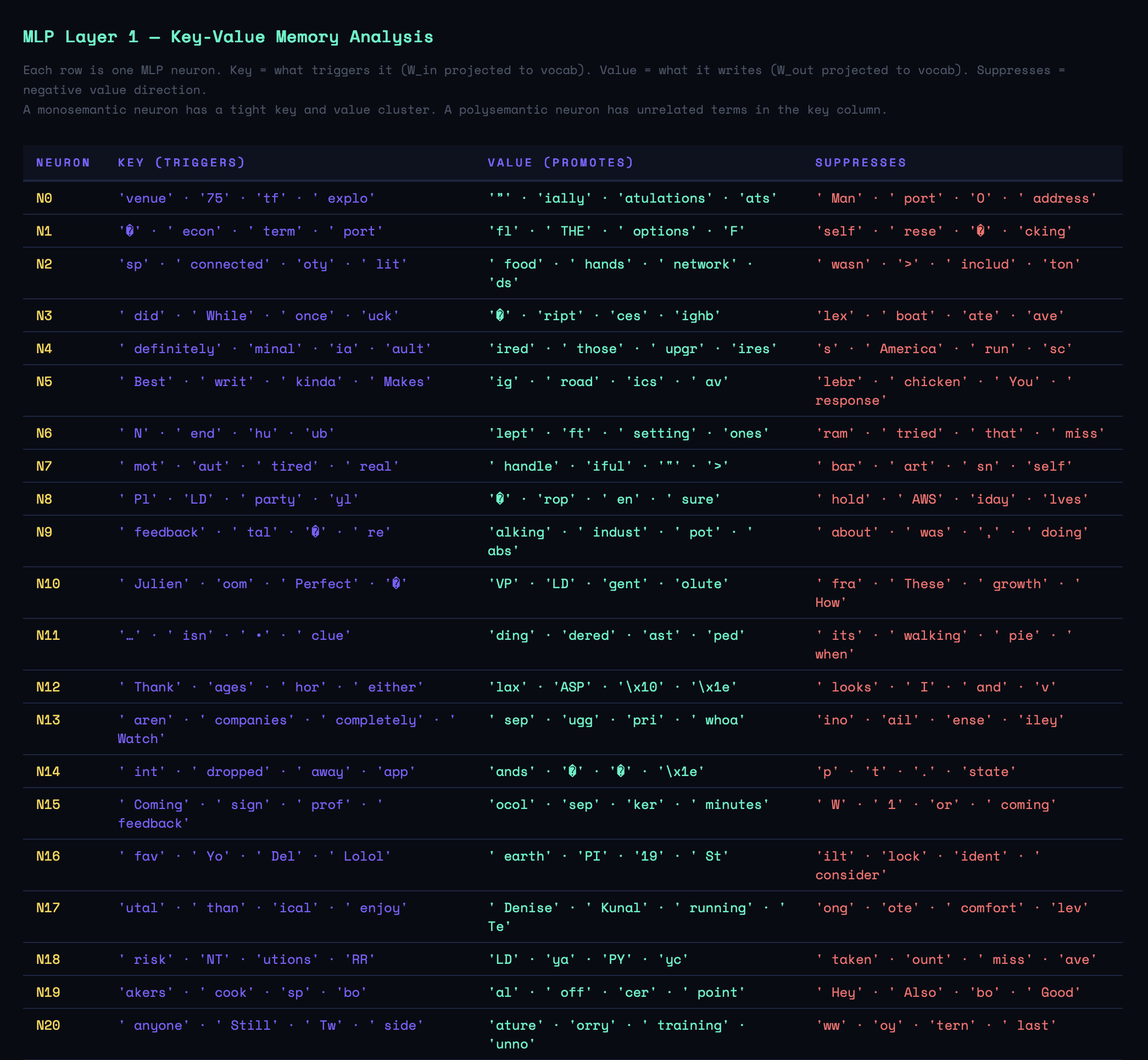
The concrete example: L1 Neuron 17.

L1 N17: key=['utal', ' than', 'ical']  →  value=[' Denise', ' Kunal', ' running']

This neuron activates in response to grammatical fragments (' than', 'ical') and writes the values ' Denise', ' Kunal', and ' running' — three completely unrelated concepts stored in the same neuron. My own name appears alongside Denise as a value because both are proper nouns that follow certain grammatical patterns in my texts, and the model has learned to pack them into the same representational direction because they're rarely active simultaneously.

Why does this happen? Mathematics. The model has 256 dimensions per layer. Your corpus contains thousands of meaningful concepts — names of people, places, topics, emotional registers, conversational functions. You cannot represent thousands of things cleanly in 256 dimensions. The solution is superposition: store multiple features in overlapping directions, accepting that individual neurons become uninterpretable, because the features are sparse enough that interference is manageable.

The implication is significant: you cannot interpret this model by reading its neurons. The internal representations are not organized to be human-readable. There is no "meeting" neuron, no "affirmation" neuron, no "scheduling" neuron. The model's knowledge is distributed across a high-dimensional geometry that neurons are poor at capturing.

This is exactly why Sparse Autoencoders (SAEs) were developed. An SAE tries to learn a higher-dimensional basis — say 4,096 features in place of 256 neurons — where concepts separate into distinct, monosemantic directions. The SAE paper from Anthropic trained on a 1-layer model and recovered interpretable features from a model that appeared completely polysemantic at the neuron level. The same approach applied to this model would be the natural next step.

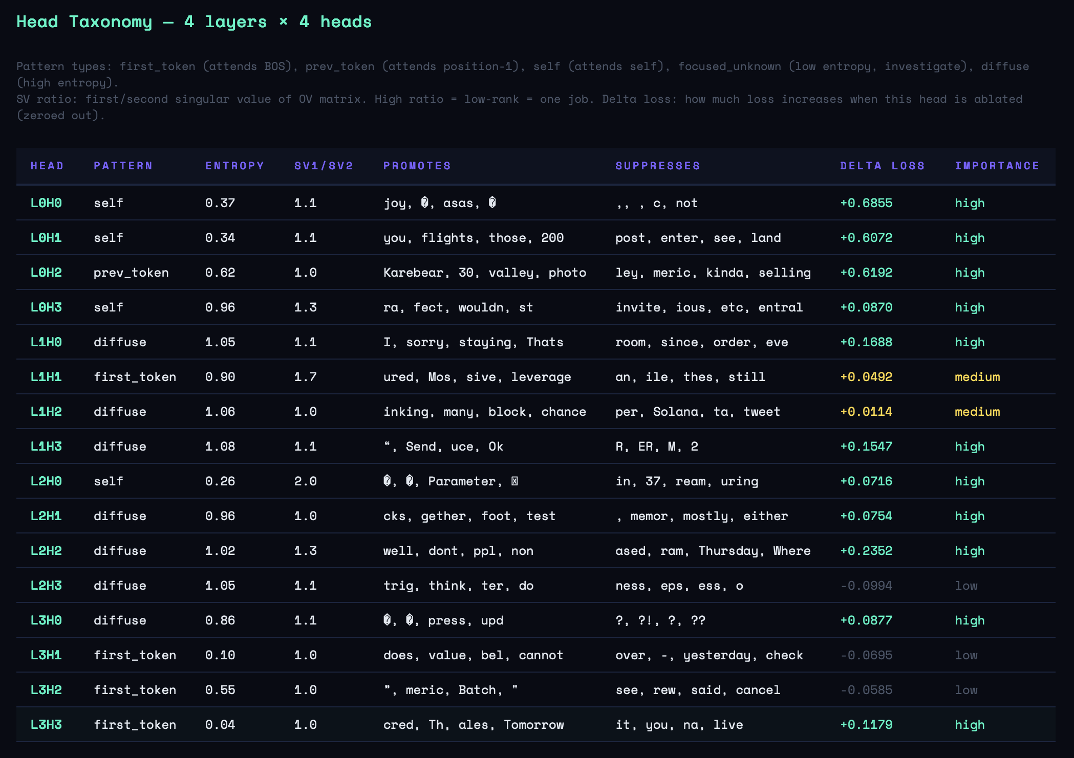
The Head Taxonomy

Here is the complete characterization of all 16 attention heads, synthesized from the entropy map, OV analysis, pattern classification, and ablation results:

Head	Pattern	Entropy	Ablation	Role
L0H0	self	0.37	+0.69 (high)	Cooperative feature encoding with L0H1
L0H1	self	0.34	+0.61 (high)	Cooperative feature encoding with L0H0
L0H2	prev_token	0.62	+0.62 (high)	Previous-token relay — structural
L0H3	self	0.96	+0.09 (med)	General self-attention mixing
L1H0	diffuse	1.05	+0.17 (high)	Context integration
L1H1	first_token	0.90	+0.05 (med)	Early speaker attention (weaker than L3)
L1H2	diffuse	1.06	+0.01 (med)	Context integration
L1H3	diffuse	1.08	+0.15 (high)	Context integration
L2H0	self	0.26	+0.07 (high)	Specialized — highest OV SV ratio (2.0)
L2H1	diffuse	0.96	+0.08 (high)	Context integration
L2H2	diffuse	1.02	+0.24 (high)	Context integration
L2H3	diffuse	1.05	-0.10 (low)	Possibly redundant
L3H0	diffuse	0.86	+0.09 (high)	Question suppression (promotes '?')
L3H1	first_token	0.10	-0.07 (low)	Speaker-tracking (secondary)
L3H2	first_token	0.55	-0.06 (low)	Speaker attention (moderate)
L3H3	first_token	0.04	+0.12 (high)	Speaker-tracking (primary — entropy 0.04)

A few things worth highlighting in this table:

L2H0 has the highest OV singular value ratio in the model (SV1/SV2 = 2.0), meaning its output is the most low-rank — it's doing the most focused single job. Its keys project to garbage tokens ('Parameter', 'ream'), suggesting it's operating on structural rather than semantic features. This head deserves more investigation.

L2H3 has negative ablation delta (-0.099) — removing it slightly improves loss. This is a head that is actively hurting average performance. It may be specialized for a behavior that the loss metric doesn't reward, or it may be a byproduct of training noise. Negative-ablation heads are one of the most interesting things to find in small models.

The L3 cluster (L3H1, L3H2, L3H3) all showing first_token patterns with varying entropy confirms that the model has dedicated its final attention layer primarily to speaker identity processing. Layer 3 is the last computation before the unembedding — it's where the model makes final adjustments before producing logits. The fact that three of four L3 heads are reading the speaker token suggests that speaker identity is the single most important feature for final prediction.

Composition Scores

The composition analysis reveals which heads are reading other heads' outputs — multi-layer circuits where the output of one head becomes meaningful input to a later head.

Top composition pairs:
  L2H3 → L3H3  (K-comp)  score=1.299
  L2H3 → L3H1  (K-comp)  score=1.285
  L2H3 → L3H2  (K-comp)  score=1.210
  L2H1 → L3H3  (K-comp)  score=1.190
  L2H0 → L3H1  (Q-comp)  score=1.181

Scores are Frobenius-norm ratios scaled by √d_model, so values above 1.0 reflect the dimensionality of the residual stream, not an error.

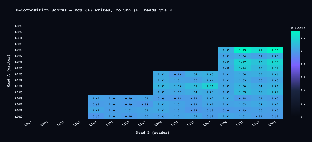
The dominant pattern is L2 heads composing with L3 heads via K-composition. K-composition means the key vectors of L3 heads are reading the value outputs of L2 heads. In plain terms: L3 heads are deciding what positions to attend to based partly on what L2 computed. Since L3 heads are primarily attending to the speaker token at position 0, this means L2 is writing information to position 0 that influences how strongly the L3 speaker-tracking heads activate.

The circuit sketch: L2 processes content words → writes contextual information to the speaker token position → L3H3 reads from the speaker token with contextual influence from L2 → late-layer prediction is conditioned on both speaker identity and L2's contextual computation.

What No Induction Heads Tells Us

Confirmed induction heads (score > 0.3): []
Previous-token heads (score > 0.5): [(0, 2)]

Induction heads are the most-studied circuit in transformer research. An induction head completes the pattern [A][B]...[A] → [B]: given a repeated sequence, it finds the previous occurrence of the current token and copies what came after it. They are considered a hallmark of in-context learning capability.

This model has no confirmed induction heads.

There are a few possible explanations. The context length is 128 tokens — short enough that many induction patterns in the training data fall outside the window. The training corpus consists of natural conversations rather than documents with longer-range structure, so the induction mechanism may not have been strongly selected for. And at 5.3M parameters, the model may simply lack sufficient capacity to develop both speaker-tracking circuits and induction circuits — it made a different trade-off.

The absence is itself informative. It suggests that conversational models and document models may develop structurally different internal organizations, even at similar scales. The dominant computational task in conversation is tracking identity, register, and pragmatic context — not completing repeated token sequences. The circuits that emerge reflect the statistics of the training data.

Potential Explorations

The findings point to four things to explore:

SAEs. The 98-100% polysemanticity result means neuron-level analysis is a dead end for this model. Training a SAE on each layer's residual stream is the obvious next move — decompose 256 dimensions into a higher-dimensional feature basis where concepts actually separate.

Speaker-tracking circuit validation. The L3H3 scrubbing experiment was invalidated by a target token selection error — the target appeared in both the clean and corrupted prompts, collapsing the logit gap to near zero. The fix is straightforward: construct a prompt pair where only the speaker token differs and the target token is unique to one prediction. That would cleanly confirm or reject the speaker-tracking hypothesis.

Induction heads. Several heads show induction scores in the 0.05-0.09 range — below the standard 0.3 threshold but not zero. The question is whether conversational data produces weak induction behavior distributed across heads rather than the clean, dedicated induction circuits found in document-trained models.

Larger model. The loss plateau at 2.83 is a capacity ceiling. An 8-layer, 8-head, 512-dimensional model (~50M parameters) on the same corpus would answer the question the current model can't: does a bigger network develop cleaner circuits and less superposition, or does it just pack more features into the same entangled geometry?

Final Thoughts

I started this project not really knowing what I was doing. I'd read a few papers, understood the basic vocabulary, and had a vague sense that interpretability was interesting. Two weekends of reading and a week of experiments later, I know significantly more — not enough to call myself a researcher, but enough to run a real pipeline, make real findings, and understand why the open questions are hard.

The thing that surprised me most was not any individual finding. It was that a 5.3M parameter model trained on text messages discovers the same computational primitives — previous-token heads, speaker-tracking specialization, superposition, polysemanticity — that appear in models a thousand times its size. Nobody told this model how GPT-2 organizes its internals. It arrived at the same solutions independently, because those solutions are what gradient descent converges on when the task is sequential prediction. That's a remarkable thing to see with your own eyes.

Here is the thing I didn't expect going in: when you run this pipeline on your own text messages, it strips away the illusion of spontaneity. You will see that your conversational habits are highly structured patterns. The model did not learn to understand you — it carved out a specific topography in high-dimensional space that mirrors your psychology. Interpreting this model becomes a strange, highly technical form of introspection.